
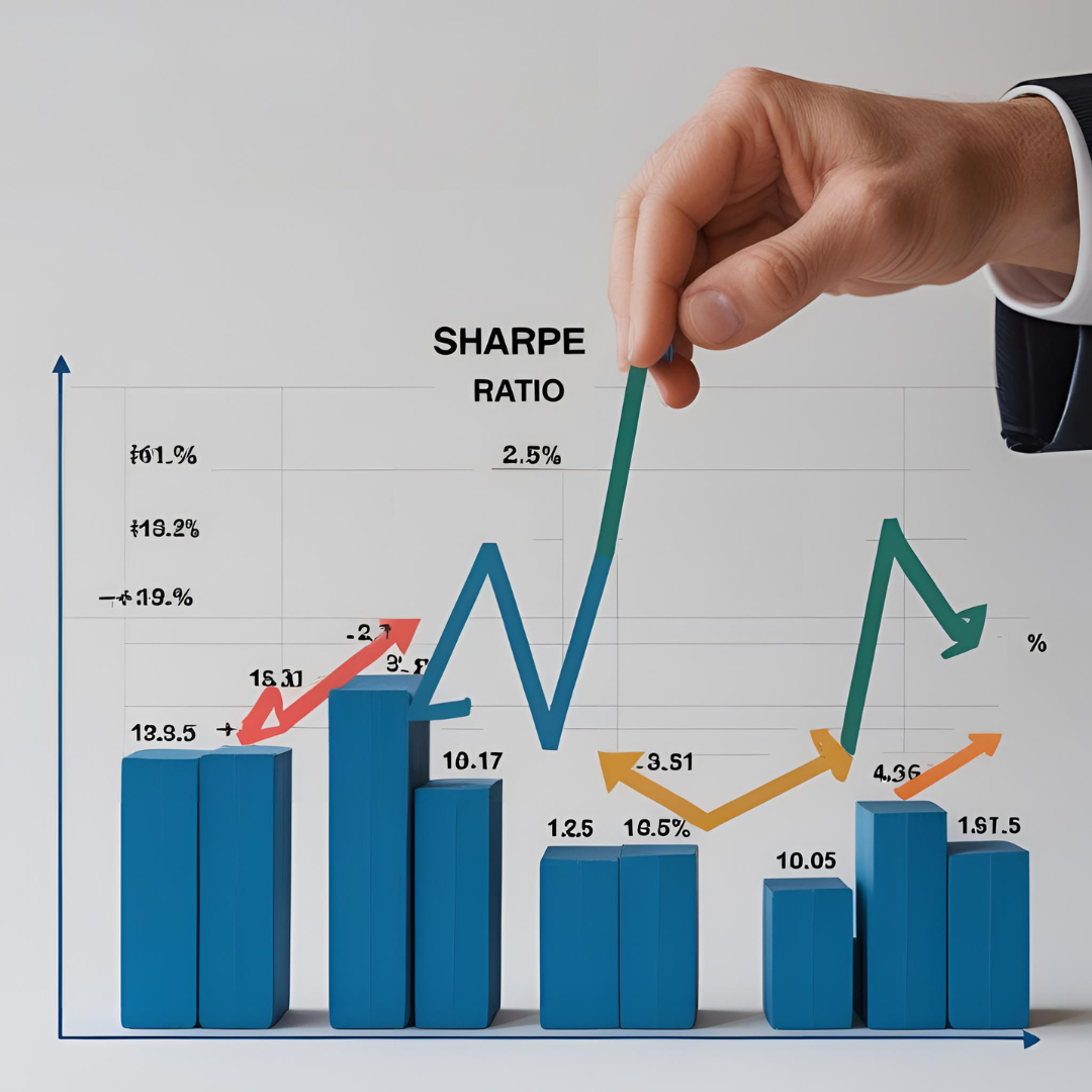
The Sharpe ratio measures a mutual fund’s risk-adjusted return by comparing its excess return (fund return minus risk-free rate) to its volatility (standard deviation of returns). A higher Sharpe indicates more return per unit of risk, helping investors assess performance efficiently.
1. Definition & Origin
The Sharpe ratio, officially known as the “reward‑to‑variability” ratio, was developed by Nobel laureate William F. Sharpe in 1966. It measures how well the return of an investment compensates an investor for the risk taken, using standard deviation as the risk proxy.
When introduced, the formula was:
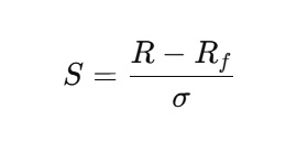
- R = expected or historical return of the fund
- R_f = risk-free rate
- σ = standard deviation of returns
A modified version, adopted in 1994 by Sharpe himself, refined the denominator to the standard deviation of excess returns (R – R_f) to adjust for risk-free variance.
2. The Formula Explained
The Sharpe ratio is calculated as:
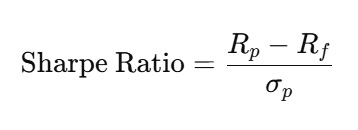
- R_p = average portfolio return over a period
- R_f = risk-free rate during the same period
- σ_p = standard deviation of the portfolio’s returns (or excess returns per revised formula)
This means the ratio expresses how many units of return are achieved per unit of volatility.
3. Why Compare to the Risk-Free Rate?
The risk-free rate acts as a benchmark—typically the return you’d get from Treasuries (e.g., T-bills in the U.S., govt securities in India). The numerator (Rp – Rf) represents the excess return, or risk premium, that the fund earns beyond what a virtually riskless investment provides.
4. Interpretation
- Sharpe > 1.0: Acceptable/good risk‑adjusted returns
- Sharpe > 2.0: Very good
- Sharpe > 3.0: Exceptional
High Sharpe: The fund delivers strong returns for each unit of risk.
Low/null Sharpe (<1): Returns may not justify volatility. If negative, the fund underperforms the risk-free alternative .
5. Practical Example
- Fund A: Rp = 12%; Rf = 3%; σ = 8% → Sharpe = (12–3)/8 = 1.125
- Fund B: Rp = 15%; Rf = 3%; σ = 12% → Sharpe = (15–3)/12 = 1.0
Despite Fund B’s higher return, Fund A wins on risk-adjusted performance.
6. Uses in Mutual Funds
- Peer Comparison
– Compare funds with similar objectives (large‑cap, debt, mid‑cap, etc.) on a level playing field. - Manager Skill Indicator
– A higher Sharpe suggests returns due to skill rather than luck or excessive risk. - Risk‑Return Trade-off
– Helps investors see if higher returns come with proportional increases in volatility. - Allocation Tool
– Evaluates how adding a fund affects overall portfolio risk‑adjusted return.
7. Limitations & Caveats
- Dependency on Normal Distribution
– Assumes returns are symmetrically distributed; ignores skewness and fat tails, so it may understate extreme risks. - Equal Weight for “Good” and “Bad” Volatility
– Penalizes upside fluctuations equally, which may misrepresent performance; Sortino ratio addresses this. - Time Period Sensitivity & Manipulation
– Cherry‑picked time frames (e.g., only months with low volatility) can artificially inflate Sharpe . - Ignores Other Risk Types
– Doesn’t account for liquidity risk, credit risk, or systemic risks; beta-based metrics (Treynor ratio) supplement it. - Unsuitable for One-Off Holdings or Illiquid Strategies
– Hedge funds, private equity with non-normal returns aren’t well represented. - Choice of Risk‑Free Benchmark
– Mismatch between Rf duration and fund horizon can skew ratios.
8. Sharpe vs. Other Metrics
| Metric | Definition |
|---|---|
| Sharpe Ratio | Excess return per unit of total volatility (σ) |
| Sortino Ratio | Excess return per unit of downside volatility |
| Treynor Ratio | Excess return per unit of systematic risk (β) |
| Alpha | Return over benchmark (risk-adjusted) |
While Sharpe looks at total volatility, Treynor isolates market risk, and Sortino focuses only on downside ‑ a more nuanced risk view.
9. Interpreting Values in Context
- Relative Measure: Sharpe alone is not enough—always benchmark against:
- Similar funds in same category
- Market benchmarks to gauge manager effectiveness
- Asset Class Differences: Equity funds typically have higher volatility, and their Sharpe expectations differ from debt or hybrid funds .
- Time Period & Frequency: Monthly vs daily return data changes σ; lower-frequency data smooths volatility, inflating Sharpe .
10. Real‑World Use & Indian Mutual Funds
- Popular in India as a quantitative criterion—often featured on mutual fund platforms like ET Money, Bajaj AMC.
- Helps investors choose mutual funds within categories—from mid‑cap to small‑cap—based on risk‑adjusted performance.
11. Working Through a Calculation
Example:
- Period: 12 months
- Monthly returns: …
- Compute:
- Average monthly return
- Monthly risk‑free rate (e.g., 0.25% from a 3% annual T‑bill)
- Compute excess monthly returns
- Derive standard deviation of those excess returns
- Annualize if needed (·√12 for σ, ·12 for average return)
The result is either a historic, realized Sharpe or an ex‑ante estimate based on forecasts.
12. Sharpe in Portfolio Construction
Sharpe aids in optimization—allocating more to funds that improve overall portfolio Sharpe. It forms the backbone of modern portfolio theory.
Modigliani measure (M²) builds on Sharpe to express risk‑adjusted return in percentage points, useful for performance comparison .
13. Common Misuses & Pitfalls
- Cherry-picking measurement periods
- Inappropriate benchmarks (unmatched Rf or peer group)
- Ignoring volatility skew (up vs down)
- Misinterpreting values outside fund category context
- Using alone, rather than alongside alpha, beta, Sortino, R‑squared.
14. Why It Matters
- Offers a quantitative, intuitive measure to compare fund quality
- Helps identify whether high returns are a result of risk control or risk concentration
- Essential in goal-based investing—matching funds to risk appetite
15. Recap
- Purpose: Measures return per unit of risk
- Formula: (Rp−Rf)/σp(R_p – R_f)/σ_p(Rp−Rf)/σp
- Interpretation: Higher is better (>1 good, >2 very good, >3 excellent)
- Comparative Use: Best used within peer groups
- Limitations: Normality assumption, symmetric volatility penalization, period-dependency
- Should be used alongside: Sortino, Treynor, alpha, beta, R²
16. Final Thoughts
The Sharpe ratio remains a foundational metric in mutual fund and portfolio evaluation. It offers clarity on risk‑adjusted returns, but must be contextualized—considering categories, time frames, data frequency, and paired analytical metrics. Used judiciously, it empowers investors to make smarter, more balanced fund selections aligned with risk tolerance and goals.
In summary: The Sharpe ratio quantifies a mutual fund’s risk‑adjusted performance by measuring excess return above a risk‑free benchmark per unit of total volatility. While intuitive and widely used, it’s most powerful when compared within peer groups and complemented by other risk metrics—and used thoughtfully in fund selection and portfolio strategy.